Super Bowl Squares COVID Edition
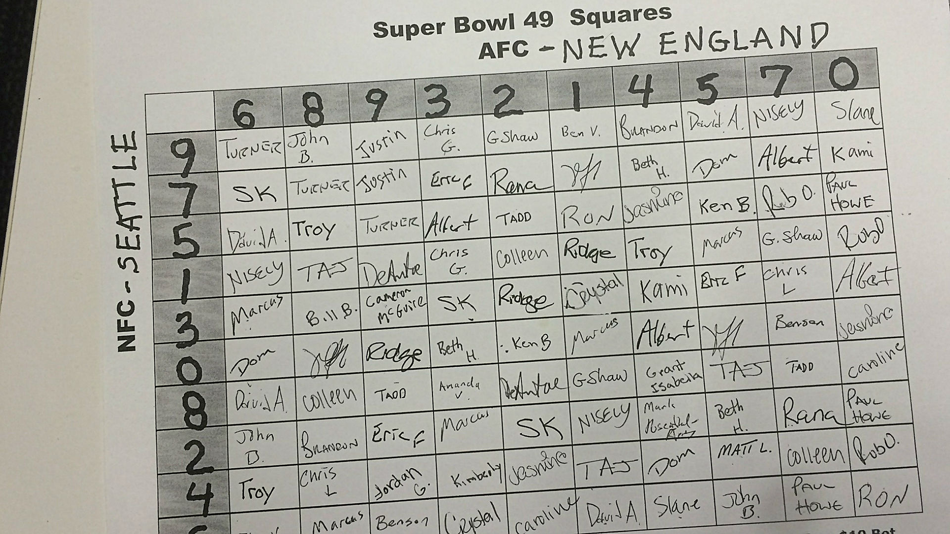
It’s that time of year again where we gather to binge on exotic dips and watch some of the most expensive commercials ever created. Also, there’s a football game. This year the merriment is likely on hold for many due to COVID, but there is a way to inject some extra excitement into your Sunday. Superbowl Squares is a bingo-esque game where participants fill out their names on a grid. Columns and rows range from 0 to 9 and correspond to the last digit of each team’s score. Those who have the correct numbers after each quarter win a prize!
This blog does not promote gambling and prizes can range from a firm handshake to fresh baked cookies.
Traditionally the numbers for columns and rows are randomly generated after names are hand written on a piece of paper, but randomly ordering the names achieves the same goal. Superbowl Squares is the best kind of game; one that requires zero skill but can still be exciting.
I decided to organize a Super Bowl Squares raffle and create my random board in R! I have a simple spreadsheet with all of the participants and the number of squares they have claimed. All squares were claimed meaning the “squares” column adds up to 100 exactly. Squares cost $20 apiece- hypothetically of course.
squares## # A tibble: 28 x 2
## participants squares
## <chr> <dbl>
## 1 Kyle 4
## 2 Dennis 5
## 3 Carlos 3
## 4 Mike 2
## 5 Parker 5
## 6 Pete 2
## 7 Papa 4
## 8 Alison 2
## 9 Julie D 4
## 10 Billy/Gena 4
## # ... with 18 more rowsBuilding a Board
The Super Bowl Squares board is simply a matrix with every combination of 0 through 9 available. I used the crossing function from the tidyr package to create a 2 column tibble with every combination of 0 - 9 possible. Each row in this tibble represents one of the 100 squares on our final board. After that all we need to do is add an additional column with a list of randomly ordered participant names. On game day I am planning a table generation ceremony where numbers are drawn out of a hat to determine the random seed.
set.seed(8017)


squares_board <- crossing(AFC = 0:9, NFC = 0:9) %>%
  mutate(name = sample(squares %>%
                         ### expand tibble to one row for each claimed square
                         uncount(squares) %>%
                         ### Turn participants column into a vector
                         pull(participants)))

head(squares_board)
## # A tibble: 6 x 3
## AFC NFC name
## <int> <int> <chr>
## 1 0 0 Kristen
## 2 0 1 Billy/Gena
## 3 0 2 Jamie
## 4 0 3 Anthony
## 5 0 4 Pete
## 6 0 5 BenRight now we have the board created in long format. We can use ggplot2 and geom_tile from here to construct the final board that will be sent to participants.
squares_board %>%
  ggplot(aes(x = factor(AFC), y = fct_rev(factor(NFC)))) +
  geom_tile(aes(fill = name), col = "black", alpha = .6) +
  geom_text(aes(label = name)) +
  scale_x_discrete(position = "top") +
  labs(x = "Kansas City", y = "Tampa Bay") +
  theme_light() +
  theme(axis.text=element_text(size=12),
        axis.title=element_text(size=14,face="bold")) +
  guides(fill = FALSE)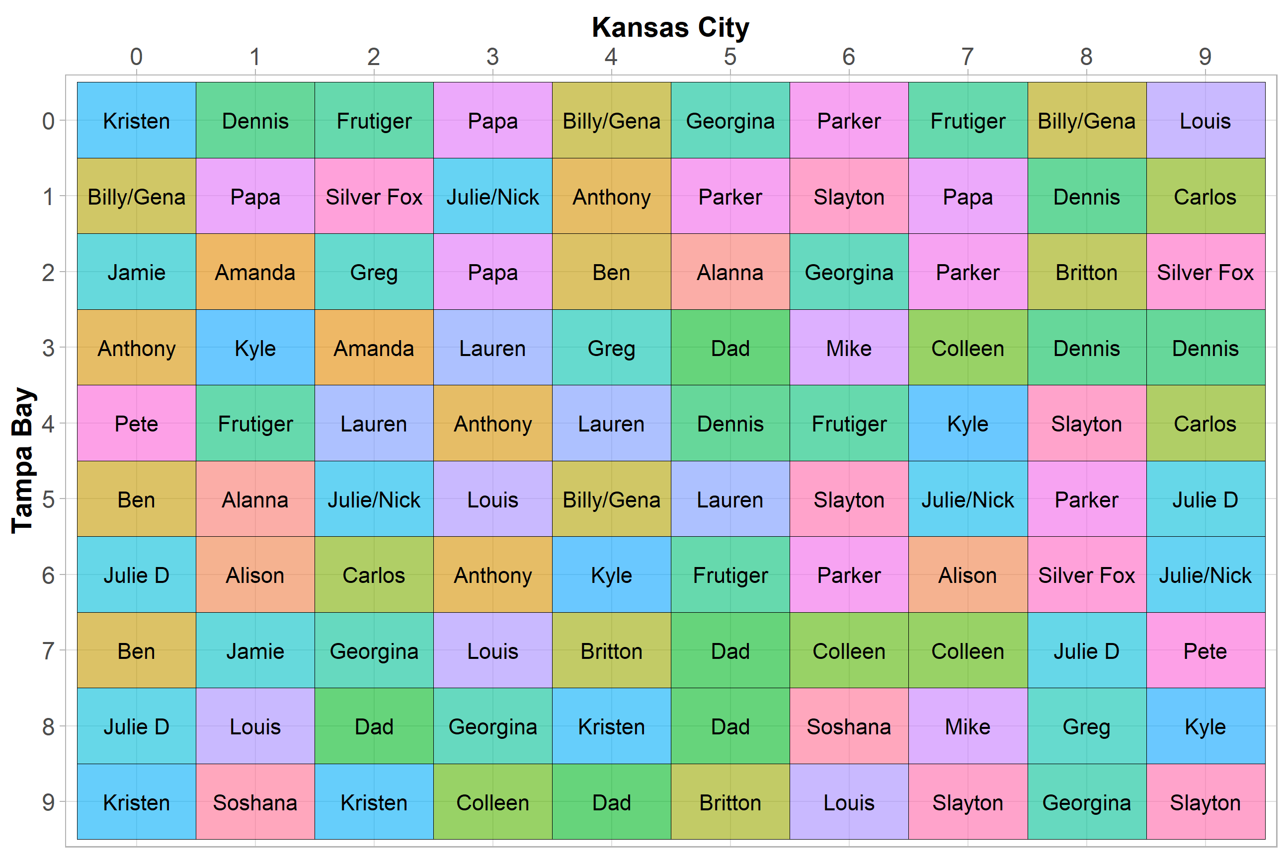
What are the best numbers?
I have a general idea which numbers on the board have the best chance of winning. Since touchdowns count as 6 points plus a 1 point field goal attempt and regular field goals count as 3, multiples of 7 and 3 are likely the best numbers. Instead of guessing I decided to scrape the score of every game ever played from the Pro Football Reference website and see what the historical results were.
## Pull score summary data
library(rvest)

content <- read_html("https://www.pro-football-reference.com/boxscores/game-scores.htm")

tables <- html_table(content)[[1]] %>%
  janitor::clean_names() %>%
  mutate(last_year = as.numeric(str_sub(last_game, -4)))


nfl_scores <- tables %>%
  select(pts_w, pts_l, count, last_year) %>%
  uncount(count) %>%
  mutate(score1 = pts_w %% 10, ## select only the last digit of each score
         score2 = pts_l %% 10,
         row_id = row_number())
This is a great opportunity to utilize the widyr package to calculate pairwise counts of our scores. I decided to filter to all scores that have occurred since 2000 to represent the modern era of NFL football.
nfl_scores_count <- nfl_scores %>%
  filter(last_year >= 2000) %>%
  pivot_longer(cols = starts_with("score")) %>%
  widyr::pairwise_count(value,row_id,sort = T) %>%
  ## Bind rows for same score tallies (this is due to a bug in widyr I believe)
  bind_rows(nfl_scores %>%
              filter(last_year >= 2000,
                     score1 == score2) %>%
              group_by(score1, score2) %>%
              tally() %>%
              ungroup() %>%
              rename(item1 = score1,
                     item2 = score2)) %>%
  group_by() %>%
  mutate(pct = (n / sum(n))) %>%
  ungroup()

head(nfl_scores_count)
## # A tibble: 6 x 4
## item1 item2 n pct
## <dbl> <dbl> <dbl> <dbl>
## 1 7 0 1206 0.0395
## 2 0 7 1206 0.0395
## 3 4 7 1133 0.0371
## 4 7 4 1133 0.0371
## 5 3 0 971 0.0318
## 6 0 3 971 0.0318Now we can easily calculate the percentages for each score combination and create our squares table as a heat map.
nfl_scores_count %>%
  mutate(pct = (n / sum(n))) %>%
  ggplot(aes(x = factor(item1), y = fct_rev(factor(item2)))) +
  geom_tile(aes(fill = n), alpha = .7) +
  geom_text(aes(label = scales::percent(pct, accuracy = .01)), fontface = "bold") +
  scale_x_discrete(position = "top") +
  scale_fill_gradientn(colors = fct_rev(RColorBrewer::brewer.pal(9,"RdYlGn"))) +
  labs(x = "", y = "", title = "Super Bowl Squares Probability",
       subtitle = "Percentages calculated from all recorded NFL scores since 2000") +
  guides(fill = FALSE) +
  theme_light() +
  theme(axis.text=element_text(size=12),
        axis.title=element_text(size=14,face="bold"))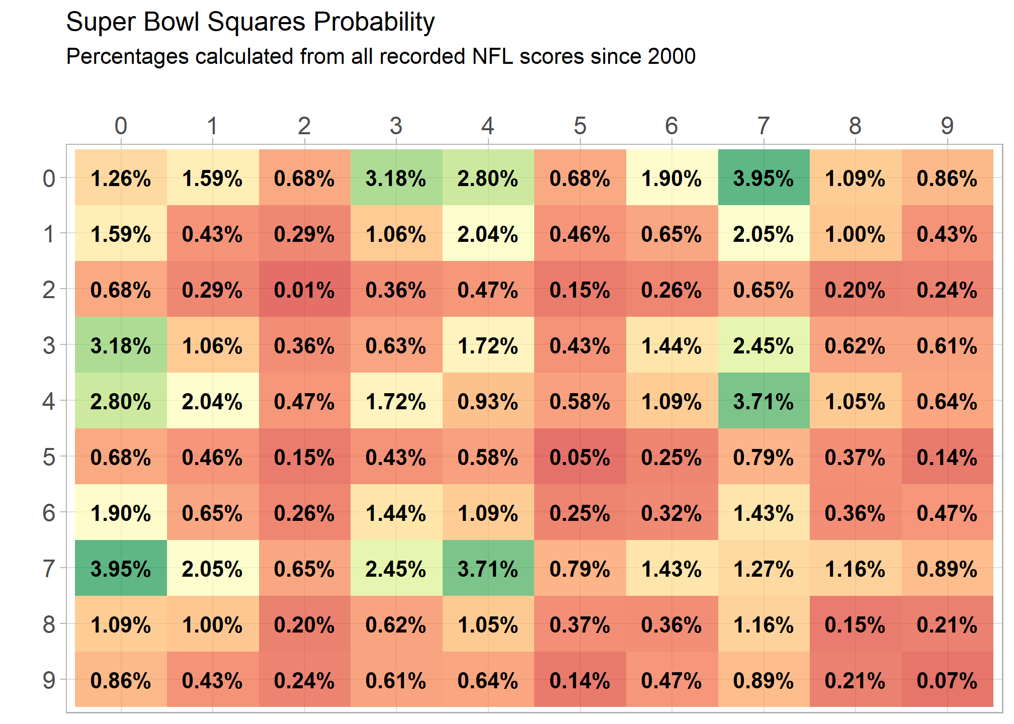
Looking at pairwise counts as a barchart shows a different perspective. Almost any combination of 0, 3, 4, or 7 is money in the bank or cookies in the basket.
nfl_scores %>%
  filter(last_year >= 2000) %>%
  pivot_longer(cols = starts_with("score")) %>%
  widyr::pairwise_count(value,row_id,sort = T,upper = F) %>%
  ## Bind rows for same score tallies (this is due to a bug in widyr I believe)
  bind_rows(nfl_scores %>%
              filter(last_year >= 2000,
                     score1 == score2) %>%
              group_by(score1, score2) %>%
              tally() %>%
              ungroup() %>%
              rename(item1 = score1,
                     item2 = score2)) %>%
  group_by() %>%
  mutate(pct = (n / sum(n))) %>%
  mutate(scores = paste0(item1,"-",item2),
         scores = fct_rev(fct_reorder(scores, n))) %>%
  ggplot(aes(x = scores, y = n)) +
  geom_col() +
  geom_text(aes(label = scales::percent(pct, accuracy = .1)), angle = 45,hjust = -.3,vjust = .1, size = 3) +
  ylim(c(0,1280)) +
  theme_minimal() +
  theme(axis.text.x = element_text(angle = 90, vjust = -.01)) +
  labs(x = "Last Digit Score Combinations", y = "count", title = "Last Digit Score Combination Totals Since 2000")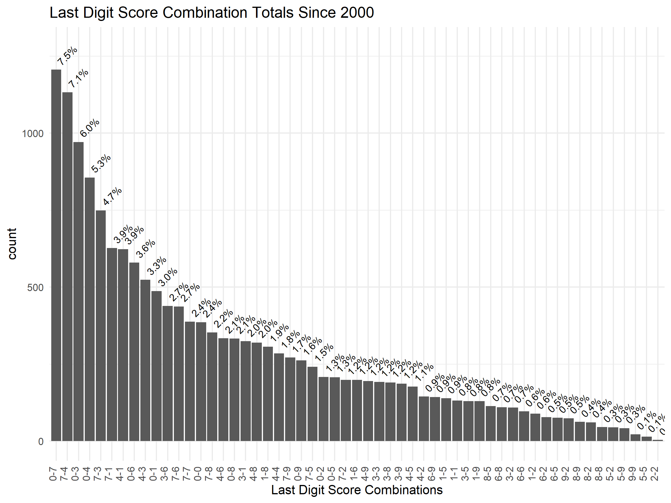
Super Bowl Squares Power Rankings
Now for what we all really care about, how likely am I to win? I combined the elongated board and NFL score probability tibbles created earlier to find out.
participant_probabilites <- squares_board %>%
  left_join(nfl_scores_count, by = c("AFC" = "item1","NFC" = "item2")) %>%
  mutate(dollars = 10,
         expected_return = dollars * pct)


participant_probabilites %>%
  group_by(name) %>%
  summarise(prob = sum(pct),
            money_spent = sum(dollars)) %>%
  mutate(name = fct_reorder(name, prob)) %>%
  ggplot(aes(x = prob, y = name, col = if_else(name == "Dennis","Y","N"))) +
  geom_point(aes(size = money_spent)) +
  geom_segment(aes(xend = prob, x = 0, yend = name, y = name)) +
  theme_minimal() +
  scale_size_continuous(labels = scales::dollar_format()) +
  scale_x_continuous(labels = scales::percent_format()) +
  labs(size = "Money Spent", y = NULL, title = "Super Bowl Squares Power Rankings",
       x = "% Change of Winning Final Prize", subtitle =  "Your's truly highlighted") +
  guides(col = FALSE)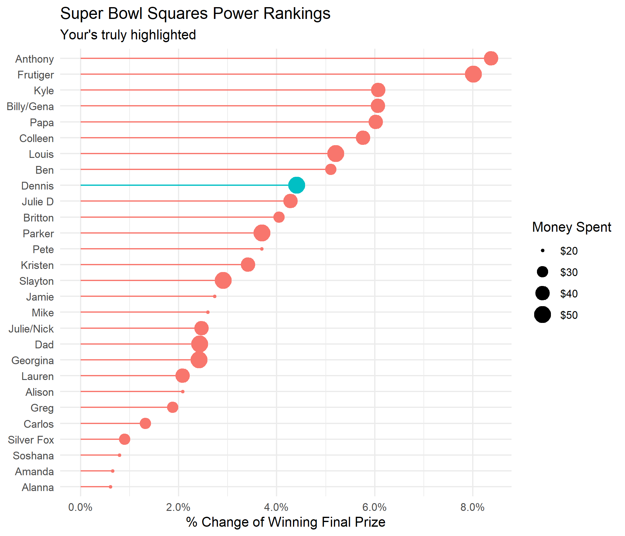
BETTER THAN MOST!

Some observations: RIP Amanda and Alannna and Pete looks like he has decent chances to win based on the amount of money he paid. This made me curios so I divided the chance of winning by the amount paid to see who got the most bang for their buck.
participant_probabilites %>%
  group_by(name) %>%
  summarise(prob = sum(pct),
            money_spent = sum(dollars),
            dollar_per_percent = sum(pct)/sum(dollars)) %>%
  mutate(name = fct_reorder(name, dollar_per_percent)) %>%
  ggplot(aes(x = dollar_per_percent, y = name, col = if_else(name == "Dennis","Y","N"))) +
  geom_point(aes(size = money_spent)) +
  geom_segment(aes(xend = dollar_per_percent, x = 0, yend = name, y = name)) +
  theme_minimal() +
  scale_size_continuous(labels = scales::dollar_format()) +
  scale_x_continuous(labels = scales::percent_format()) +
  theme_minimal() +
  labs(size = "Money Spent", y = NULL, title = "Super Bowl Squares Power Rankings",
       x = "% Gain Per Dollar Spent", subtitle =  "Your's truly highlighted") +
  guides(col = FALSE)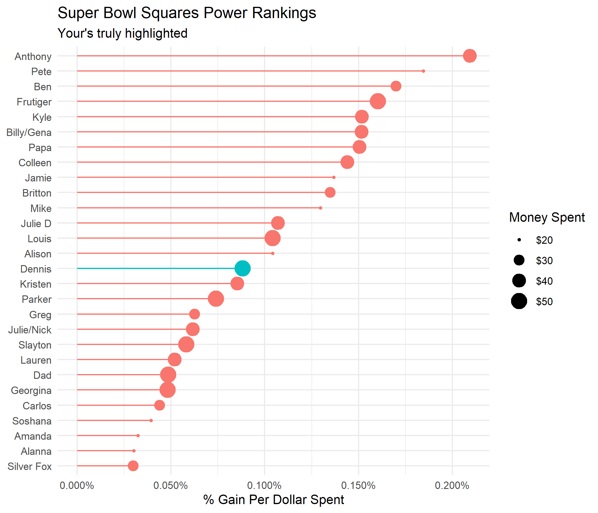
Aaaand I look considerably worse from an efficiency standpoint.

Anthony is clearly the top ranked player in terms of overall chances to win and efficiency of dollars spent. Per usual, I am rooting for chaos to ensue. Give us a safety and bring down the 0, 3, 4, and 7 holders in their ivory towers!